Examples

This page helps choose which example to run. Each script writes CSV data, a short text report, and figures into its output directory. Use --out-dir for tutorial runs so generated data does not mix with source files.

Recommended order

1. 01_ir_noninteracting_gf: check sparse-IR transforms on a known G0.

2. 02_cell_average_convergence: see why diagonal cell averages matter.

3. 03_g0w0_takada_curve: compare truncated G0W0, no-truncation G0W0, and the Takada projection.

4. 04_g0w0_gw0_scgw_curve: compare G0W0, GW0, and scGW density curves.

5. 05_screening_phonon_controls: isolate electronic screening and phonon enhancement controls.

6. 06_g0w0_w_gap_diagnostics: inspect fixed G0W0 interaction and gap functions.

7. 07_gw0_scgw_w_gap_diagnostics: inspect GW0/scGW interactions and gap functions.

8. 08_tc_vs_density: build a Tc curve from \(\lambda(T)=1\) using same-density cooling restarts.

9. 09_multi_phonon_modes: repeat the G0W0/GW0/scGW density-curve comparison with an explicit three-pole phonon dielectric factor.

How to read outputs

The CSV files are the machine-readable result. The text report records the question, method settings, and a compact result summary. Figures are meant for quick inspection.

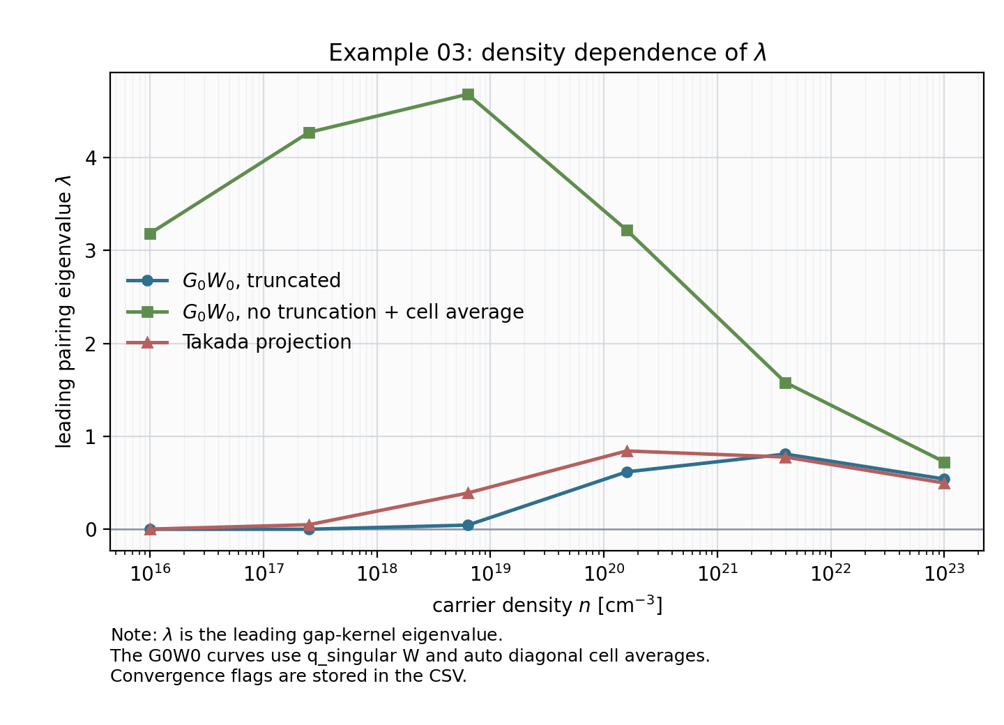
Example 03 output preview. Treat figures like this as a visual summary; use the CSV columns and convergence flags when quoting numbers.

For GW0 and scGW examples, always check the SCF convergence columns before interpreting lambda. Some tutorial scripts intentionally keep unconverged rows so a full curve can show where convergence becomes difficult. Use --fail-unconverged when you want non-convergence to stop the run.

Practical tips

Use --out-dir to keep generated files outside the repository:

python examples/01_ir_noninteracting_gf/run.py --out-dir /tmp/migdal-example01

For MPI examples:

mpirun -n 2 python examples/03_g0w0_takada_curve/run.py \
  --out-dir /tmp/migdal-example03

Use python <example>/run.py --help for the full option list. The examples share many grid and sparse-IR flags, but each script exposes only the controls needed for its question.

Example 9 uses STOParams.phonon_to_poles_cm and STOParams.phonon_lo_zeros_cm to switch the lattice factor from the default single-pole model to the three-pole multipole representation described in Bare interaction and screening. The default run scans six log-spaced densities from \(10^{23}\) to \(10^{16}\,\mathrm{cm}^{-3}\) and writes multi_phonon_modes.csv, multi_phonon_modes.txt, and multi_phonon_modes.png. Check the GW0/scGW SCF convergence columns before using the reported lambda values.

For a guided path through these scripts, start with Choose a method. For the meaning of CSV columns, see CSV columns.