Theory

This page is the self-contained theory guide for Migdal. It explains the physical problem, the equations being solved, and the numerical choices used by the public drivers.

Migdal is intentionally narrow: it studies an isotropic one-band model for an SrTiO3-like polar semiconductor, then compares four ways of estimating the linearized pairing strength. The goal is not to be a general-purpose electron-phonon package. The goal is to make a controlled comparison between fixed-W0, self-consistent, and projected pairing calculations on the same radial model.

The basic question

At a chosen carrier density and temperature, the code asks whether a normal metal is close to a superconducting instability. In practice it computes a linearized gap eigenvalue. In Example 08, the transition temperature is estimated from

\[ \lambda(T_{\mathrm{c}}) = 1. \]

The four public drivers answer this question at different levels:

• G0W0 uses the noninteracting \(G_0\), a fixed \(W_0\), and the sparse-IR radial gap eigenproblem.

• GW0 solves the normal-state \(G\) self-consistently, keeps \(W_0\) fixed, and then runs the same sparse-IR gap solver.

• ScGW solves both \(G\) and \(W\) self-consistently before the same gap solve.

• TakadaProjection is a dense projected comparison solver with its own eV/Angstrom units and projected kernel.

The approximation hierarchy is:

Driver	Normal propagator	Screened interaction	Pairing problem
G0W0	Noninteracting \(G_0\)	Fixed \(W_0\) from analytic or numerical \(G_0G_0\) polarization	Sparse-IR radial gap solver
GW0	Self-consistent \(G\)	Same fixed \(W_0\) as the setup point	Sparse-IR radial gap solver
ScGW	Self-consistent \(G\)	Self-consistent RPA \(W\) from the current bubble	Sparse-IR radial gap solver
TakadaProjection	Projected \(G_0\) comparison setup	Dense projected \(W_0\)	Dense projected eigenproblem

This is a Migdal-Eliashberg style calculation in imaginary frequency: the interaction is dynamical, the normal propagator is a Matsubara Green’s function, and the pairing problem is an eigenvalue problem rather than a fitted BCS coupling constant (Migdal 1958; Eliashberg 1960). The historical background is the screened electron-phonon interaction of Bardeen and Pines (1955), the normal-state approximation of Migdal (1958), and Eliashberg’s finite-temperature gap equations (1960). The Takada driver is a separate projected comparison inspired by Takada’s work on n-type SrTiO3 (1980). For a first numerical comparison of these approximations, use Example 03 for G0W0 versus Takada and Example 04 for G0W0, GW0, and scGW.

Units and one-band model

The sparse-IR radial drivers use atomic units internally:

Quantity	Internal unit
Energy	Hartree
Length	Bohr
Momentum	\(\mathrm{Bohr}^{-1}\)
Inverse temperature \(\beta\)	\(\mathrm{Hartree}^{-1}\)

Public carrier densities are spin-summed densities in \(\mathrm{cm}^{-3}\). The drivers convert them to \(\mathrm{Bohr}^{-3}\) before constructing the radial Fermi sphere.

The electronic band is parabolic,

\[ \varepsilon(k) = a k^2, \qquad a = \frac{1}{2m_{\mathrm{eff}}}, \]

where m_eff is measured in electron-mass units. At zero temperature,

\[ n = 2\int_{|k|<k_{\mathrm{F}}}\frac{\mathrm{d}^3 k}{(2\pi)^3} = \frac{k_{\mathrm{F}}^3}{3\pi^2}, \qquad \mu_0 = a k_{\mathrm{F}}^2. \]

At finite temperature, the noninteracting density is

\[ n(\mu,T) = \frac{1}{\pi^2} \int_0^\infty \mathrm{d}k\, k^2 f(a k^2 - \mu), \qquad f(x) = \frac{1}{\mathrm{e}^{\beta x}+1}. \]

model.get_mu solves this scalar equation for the reference chemical potential. In GW0 and ScGW, the chemical potential is solved again inside the self-consistent loop because the interacting density depends on the current self-energy.

TakadaProjection is the unit exception. It works in eV and Angstrom units and uses the dimensionless variable \(x = \xi/E_{\mathrm{F}}\).

Bare interaction and screening

The radial sparse-IR drivers build a Coulomb interaction multiplied by a polar phonon dielectric factor,

\[ V_{\mathrm{c}}(q) = \frac{4\pi}{\epsilon_\infty q^2}, \]

\[ V_{\mathrm{ph}}(q,\mathrm{i}\nu_n) = \frac{\nu_n^2 + \omega_{\mathrm{TO}}(q)^2} {\nu_n^2 + \omega_{\mathrm{LO}}(q)^2}, \qquad V_{\mathrm{tot}}(q,\mathrm{i}\nu_n) = V_{\mathrm{c}}(q) V_{\mathrm{ph}}(q,\mathrm{i}\nu_n). \]

Here \(V_{\mathrm{tot}}\) is the bare interaction denoted \(\mathcal{V}\) in the STO-GW manuscript.

This is the default single-pole representation. If STOParams is given both phonon_to_poles_cm and phonon_lo_zeros_cm, the code instead uses the multipole factor

\[ V_{\mathrm{ph}}(q,\mathrm{i}\nu_n) = \prod_j \frac{\nu_n^2 + \omega_{\mathrm{TO},j}(q)^2} {\nu_n^2 + \omega_{\mathrm{LO},j}^2}. \]

By default the multipole poles are q-independent. The opt-in phonon_to_omega2_disp_cm2_a2 field gives squared-frequency TO dispersion, \(\omega_{\mathrm{TO},j}(q)^2 = \omega_{\mathrm{TO},j}(0)^2 + \beta_j q_A^2\), with \(q_A\) in Angstrom\(^{-1}\); the LO zeros remain fixed. If phonon_to_omega2_cap_cm2 supplies a finite cap \(\Omega_{\mathrm{cap},j}^2\) for a mode with positive \(\beta_j\), the code instead uses

\[ \omega_{\mathrm{TO},j}(q)^2 = \omega_{\mathrm{TO},j}(0)^2 + \Delta_j \frac{q_A^2}{q_A^2 + q_{c,j}^2}, \qquad \Delta_j = \Omega_{\mathrm{cap},j}^2 - \omega_{\mathrm{TO},j}(0)^2, \qquad q_{c,j}^2 = \frac{\Delta_j}{\beta_j}. \]

This keeps the same small-q slope, \(\omega_{\mathrm{TO},j}(q)^2 = \omega_{\mathrm{TO},j}(0)^2 + \beta_j q_A^2 + O(q_A^4)\), but approaches the finite cap at large q. Use math.inf for modes that should remain uncapped.

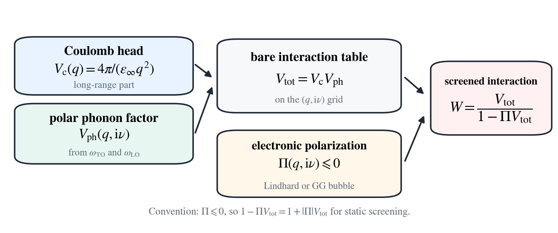
The lattice part builds \(V_{\mathrm{tot}}=V_{\mathrm{c}}V_{\mathrm{ph}}\) first. The electronic polarization \(\Pi\) then enters the RPA/GW denominator that defines the screened interaction \(W\) used by the self-energy and gap kernels.

This is the imaginary-axis form of a polar dielectric response. At zero bosonic frequency the phonon factor reduces the long-range Coulomb interaction by the large static dielectric response. At high frequency the phonon factor approaches one, leaving the Coulomb interaction screened only by \(\epsilon_\infty\).

The longitudinal mode is set by the Lyddane-Sachs-Teller relation,

\[ \frac{\omega_{\mathrm{LO}}(0)^2}{\omega_{\mathrm{TO}}(0)^2} = \frac{\epsilon_0}{\epsilon_\infty}. \]

For the multipole representation this endpoint condition becomes

\[ \prod_j \frac{\omega_{\mathrm{LO},j}^2}{\omega_{\mathrm{TO},j}^2} = \frac{\epsilon_0}{\epsilon_\infty}. \]

When omega_t_disp_cm_a2 is nonzero, model.get_Vph_q evaluates the transverse mode in Angstrom units and converts it back to the atomic-unit radial grid. The legacy single-pole convention uses

\[ \epsilon_0(q) = \epsilon_0 \left[\frac{\omega_{\mathrm{TO}}(0)}{\omega_{\mathrm{TO}}(q)}\right]^2, \]

so \(\omega_{\mathrm{LO}}(q)=\omega_{\mathrm{TO}}(q)\sqrt{\epsilon_0(q)/\epsilon_\infty}\) remains equal to the zone-center longitudinal value. The exact no-phonon limit \(\epsilon_0 = \epsilon_\infty\) is handled separately so that \(V_{\mathrm{ph}}=1\) even if a transverse dispersion parameter is present. The legacy omega_t_disp_cm_a2 field remains single-pole only; q-dependent multipole calculations use phonon_to_omega2_disp_cm2_a2, optionally with finite phonon_to_omega2_cap_cm2 entries. In that multipole case the static endpoint is

\[ \epsilon_0(q) = \epsilon_\infty \prod_j \frac{\omega_{\mathrm{LO},j}^2} {\omega_{\mathrm{TO},j}(q)^2}. \]

The code requires the sampled q grid to keep the TO modes below the LO zeros and to keep \(\epsilon_0(q) > \epsilon_\infty\).

Example 05 is the shortest way to see this part of the model in action: it turns electronic screening and phonon enhancement on and off, then records how the leading pairing eigenvalue changes.

The screened interaction is the RPA/GW form used in Hedin-style screened interaction calculations (Hedin 1965),

\[ W(q,\mathrm{i}\nu_n) = \frac{V_{\mathrm{tot}}(q,\mathrm{i}\nu_n)} {1 - \Pi(q,\mathrm{i}\nu_n)V_{\mathrm{tot}}(q,\mathrm{i}\nu_n)}. \]

The code uses the electron-gas sign convention \(\Pi \le 0\). With this convention, static electronic screening makes the denominator look like \(1+|\Pi|V_{\mathrm{tot}}\) for ordinary positive interactions. denom_policy only controls what happens when the sampled denominator becomes too small; it does not change this sign convention.

Polarization

For fixed-W0 calculations, G0W0 and GW0 usually use the finite-temperature Lindhard polarization (Lindhard 1954). The zero-temperature electron gas has the useful limit

\[ \Pi_0(q=0,\mathrm{i}\nu=0) = -\frac{m_{\mathrm{eff}} k_{\mathrm{F}}}{\pi^2}, \]

with spin degeneracy included. At nonzero \(q\) and imaginary frequency, the code uses stable closed forms in model.get_Pi0, including special handling near \(q=0\) and \(q=2k_{\mathrm{F}}\).

The finite-temperature implementation is not a brute-force two-dimensional momentum integral. It uses the thermal-smearing identity

\[ \Pi_\beta(q,\mathrm{i}\nu;\mu) = \int_0^\infty \mathrm{d}E\, [-f'(E-\mu)]\, \Pi_{T=0}\left(q,\mathrm{i}\nu;k_{\mathrm{F}}=\sqrt{E/a}\right). \]

This is mathematically useful because the difficult \(q=0\) and \(2k_{\mathrm{F}}\) limits stay inside the same stable zero-temperature formula. The quadrature is taken in the variable \(k_{\mathrm{F}}(E)=\sqrt{E/a}\), in which the \(E=0\) band edge is analytic, and the window is split at \(k_{\mathrm{F}}(\mu)\), where the thermal weight is concentrated, and at the Kohn point \(k_{\mathrm{F}}=q/2\), where the zero-temperature kernel has its \(2k_{\mathrm{F}}\) kink, whenever those points lie inside the window; the non-smooth points then sit at panel endpoints and the fixed-order Gauss-Legendre rule stays accurate. When \(\beta\mu\) is very large, model.get_Pi0_finite_T falls back to the zero-temperature formula to avoid resolving an extremely narrow thermal window.

For a visual diagnostic of the resulting screened interaction, compare Example 06 for fixed-W0 G0W0 with Example 07 for GW0/scGW.

In ScGW, the polarization is rebuilt from the current Green’s function using the imaginary-time bubble. In radial form the code evaluates

\[ \Pi(q,\tau) = -\frac{1}{2\pi^2 q} \int \mathrm{d}k\, k\,G(k,\tau) \int_{|k-q|}^{k+q} \mathrm{d}p\,p\,G(p,\beta-\tau), \]

with an analytic \(q\to 0\) limit. The Matsubara result is then symmetrized and checked before building the next \(W\).

The default scGW low-q stabilization is a continuation, not a new polarization model. With pi_low_q_policy="asymptotic", finite bosonic frequencies are continued below \(q_{\mathrm{ref}}=q_{\mathrm{low}} k_{\mathrm{F}}\) as

\[ \Pi(q,\mathrm{i}\nu_n) = \left(\frac{q}{q_{\mathrm{ref}}}\right)^2 \Pi(q_{\mathrm{ref}},\mathrm{i}\nu_n), \qquad \nu_n \ne 0, \]

consistent with charge conservation at long wavelength. The static component is held constant below \(q_{\mathrm{static}}=q_{\mathrm{static,low}} k_{\mathrm{F}}\):

\[ \Pi(q,0) = \Pi(q_{\mathrm{static}},0). \]

If q_static_low_factor is not set, the code uses the same factor as q_low_factor. Setting pi_low_q_policy="none" skips this continuation and uses the sampled bubble directly.

Green’s functions and density

The normal-state Green’s function convention is

\[ G(k,\mathrm{i}\omega_n) = \frac{1} {\mathrm{i}\omega_n - [\varepsilon(k)-\mu] - \Sigma(k,\mathrm{i}\omega_n)}. \]

The sampled Matsubara axis is always axis 1 in arrays with shape (nk, nw). Fermionic frequencies are reverse-index paired,

\[ \omega_i = -\omega_{N-1-i}, \]

which is why many symmetry checks in the code reverse the second axis.

For density constraints, the production convention is the high-frequency corrected endpoint formula

\[ n_k = 2 f(\varepsilon_k-\mu) - 2 [G-G_0](\tau=\beta^-). \]

The noninteracting occupation is known analytically, while only the correlated difference is transformed to the endpoint. This avoids making the sparse-IR transform reproduce the full \(1/(\mathrm{i}\omega)\) tail of \(G\) just to count particles. The radial density is then

\[ n = \int_0^\infty \frac{\mathrm{d}k\,k^2}{2\pi^2}\,n_k. \]

For direct checks, the code can also use \(n_k=-2G(\beta^-)\), but the corrected form is the default for the self-consistent drivers.

Radial convolution

The model is isotropic, so a three-dimensional convolution can be reduced to one radial integral. For a target momentum \(k\) and source momentum \(p\),

\[ q = |\mathbf{k}-\mathbf{p}|, \qquad |k-p| \le q \le k+p. \]

Using \(\mathrm{d}^3p/(2\pi)^3\) normalization,

\[ \int\frac{\mathrm{d}^3p}{(2\pi)^3} F(p) W(|\mathbf{k}-\mathbf{p}|) = \frac{1}{(2\pi)^2 k} \int_0^\infty \mathrm{d}p\,p F(p) \int_{|k-p|}^{k+p} \mathrm{d}q\,q W(q), \]

for \(k>0\), with an analytic \(k\to0\) row handled separately. This formula is the reason radial.py precomputes primitives of \(qW(q)\) and evaluates interval differences instead of performing angular quadrature in every matvec.

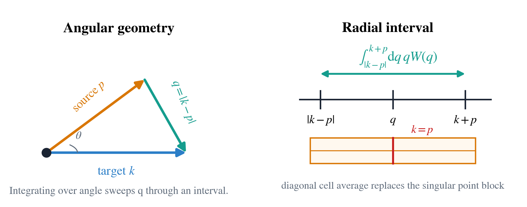
For fixed radial momenta \(k\) and \(p\), changing the angle between the vectors sweeps the transfer momentum through \(q\in[|k-p|, k+p]\). This is the geometric reason the implementation stores primitives of \(qW(q)\) and evaluates interval differences. The diagonal block \(k=p\) is also where the Coulomb-head primitive contains the logarithmic singular point, so the q_singular path needs a finite-cell average rather than a point value.

The Coulomb head is the main numerical complication. If

\[ W(q) = \frac{A}{q^2} + W_{\mathrm{reg}}(q), \]

then the radial integrand contains

\[ qW(q) = \frac{A}{q} + qW_{\mathrm{reg}}(q), \]

and the singular part has the exact primitive

\[ \int_{|k-p|}^{k+p} \frac{\mathrm{d}q}{q} = \log(k+p) - \log|k-p|. \]

This is finite away from the diagonal but diverges at the point block \(k=p\). The continuum integral is still integrable after averaging over a finite radial cell. Therefore q_interp_mode="q_singular" requires diagonal cell averages: the code replaces only the self-cell radial block by a cell average. It does not change the Matsubara transform, the definition of \(W\), or the source array.

Example 02 quantifies the convergence benefit of diagonal cell averaging by comparing point-diagonal and cell-average treatments across a sequence of radial grids. In the q_singular path, the Coulomb head is separated so that the singular part is integrated analytically and only the regular residual is interpolated.

For an unscreened Coulomb tail the coefficient is simply the Coulomb head. For the screened interaction the low-q coefficient must be inferred after the RPA denominator is applied. Write

\[ V_{\mathrm{tot}}(q,\mathrm{i}\nu_n) = \frac{B(\mathrm{i}\nu_n)}{q^2} + V_{\mathrm{reg}}(q,\mathrm{i}\nu_n), \]

and expand the polarization as

\[ \Pi(q,\mathrm{i}\nu_n) = P_0(\mathrm{i}\nu_n) + C(\mathrm{i}\nu_n)q^2 + O(q^4). \]

Then the head of \(W=V_{\mathrm{tot}}/(1-\Pi V_{\mathrm{tot}})\) is

\[ A_W(\mathrm{i}\nu_n)=\lim_{q\to0} q^2 W(q,\mathrm{i}\nu_n). \]

If \(P_0\ne0\), the static metallic response screens away the \(1/q^2\) tail and \(A_W=0\). If \(P_0=0\), as expected at nonzero bosonic Matsubara frequency by charge conservation, the remaining coefficient is

\[ A_W(\mathrm{i}\nu_n)= \frac{B(\mathrm{i}\nu_n)} {1-C(\mathrm{i}\nu_n)B(\mathrm{i}\nu_n)}. \]

The production q_singular_head_policy="pi_head" path uses this polarization head construction together with the analytic \(V_{\mathrm{tot}}\) head supplied by the STO model. The fit_w policy instead fits \(q^2W\) directly from sampled low-q rows; it is useful as a diagnostic of the singular-head construction but is not the default.

Sparse-IR sampling

At low temperature, direct Matsubara grids become large because many frequencies are needed to cover both the Fermi scale and high-energy tails. The intermediate representation (IR) compresses imaginary-time and Matsubara Green’s functions using a basis controlled mainly by the sparse-IR construction of Shinaoka et al. (2017) and Wallerberger et al. (2023), with sparse sampling in the spirit of Li et al. (2019),

\[ \Lambda = \beta\omega_{\mathrm{max}}. \]

The idea is to start from the spectral representation of a finite-temperature propagator. After rescaling \(\tau\) and real frequency to dimensionless domains, the kernel that connects spectral weight to \(G(\tau)\) has a singular-value decomposition. The IR basis functions are the left and right singular functions of that kernel. A Green’s function is represented as

\[ G(\tau) \approx \sum_{\ell=0}^{L-1} G_\ell U_\ell(\tau), \]

or, on Matsubara frequencies,

\[ G(\mathrm{i}\omega_n) \approx \sum_{\ell=0}^{L-1} G_\ell \hat U_\ell(\mathrm{i}\omega_n), \]

with fermionic or bosonic basis functions chosen according to the statistic of the quantity being transformed. The singular values decay rapidly enough that the required basis size is controlled mainly by \(\Lambda\) and the requested tolerance. This is why sparse-IR remains practical at low temperature: the sample count grows much more gently than a dense uniform Matsubara grid.

Sparse sampling adds another ingredient. Instead of storing every Matsubara frequency or every imaginary-time point, the code uses selected tau and Matsubara samples from which the IR coefficients can be reconstructed. The dense matrices in FreqGrid are the resulting transformations between sampled values and IR coefficients.

freq.FreqGrid stores the sampled fermionic and bosonic frequencies, sampled imaginary times, and dense transform matrices between those sampled axes. The rest of the code treats these arrays as ordinary matrices. This is deliberate: the radial kernels can focus on momentum integrals, while FreqGrid owns the frequency/tau convention.

Example 01 is the direct tutorial check for this section. It builds a FreqGrid, evaluates a known noninteracting \(G_0\) on the sampled fermionic Matsubara points, transforms \(G_0(\mathrm{i}\omega_n)\) to \(G_0(\tau)\) and back, then plots the round-trip error. If this example fails, later gap calculations are not yet worth interpreting.

Two implementation details matter when reading the code:

Detail	Why it exists
Axis 1 is always Matsubara or tau.	Serial arrays and MPI rank-local row blocks use the same convention.
Reverse-frequency pairing is checked explicitly.	Normal self-energies and gap functions are projected onto the expected imaginary-axis symmetry.

Linearized gap eigenproblem

The sparse-IR drivers solve the pairing instability as an eigenproblem. In schematic continuum notation, the singlet linearized equation has the form

\[ \lambda\Delta(k,\mathrm{i}\omega_n) \sim -\sum_m\int \mathrm{d}p\, W(k,p;\mathrm{i}\omega_n-\mathrm{i}\omega_m) G(p,\mathrm{i}\omega_m)G(p,-\mathrm{i}\omega_m) \Delta(p,\mathrm{i}\omega_m), \]

with the same radial angular reduction used by the normal self-energy. The code does not build this dense matrix. Instead, gap.solve_gap supplies a matrix-vector product to PySCF’s Davidson solver.

The packed vector stores the scaled gap variable

\[ \tilde{\phi}(k,\mathrm{i}\omega_n) = k\,\Delta(k,\mathrm{i}\omega_n). \]

The factor of \(k\) removes the removable \(1/k\) singularity in the radial formula and keeps the matvec finite near the origin. For a trial vector, the source is

\[ S(k,\mathrm{i}\omega_n) = G(k,\mathrm{i}\omega_n)G(k,-\mathrm{i}\omega_n)\tilde{\phi}(k,\mathrm{i}\omega_n). \]

The numerical operator sent to Davidson is

\[ M\tilde{\phi} = -\widetilde{\Sigma}[S], \]

where \(\widetilde{\Sigma}=k\Sigma\) is the scaled radial self-energy convolution. In radial.get_sigma, the self-energy convention already contains the usual minus sign of the Matsubara self-energy convolution. gap.solve_gap therefore applies the explicit extra minus sign shown above before passing the matvec to Davidson. Davidson returns raw eigenvalues \(\eta\). The code selects the root with the smallest real raw eigenvalue and reports

\[ \lambda = -\operatorname{Re}(\eta_{\mathrm{selected}}). \]

This sign convention is easy to miss when reading only the CSV output. Use the reported lambda for comparisons and for the \(\lambda(T)=1\) crossing.

Example 03 shows this reported eigenvalue as a density curve, while Example 06 and Example 07 save gap-function diagnostics so the eigenvector shape can be inspected instead of treating lambda as a black-box number.

Frequency truncation is optional. If it is enabled, gap.get_active_w keeps all reverse-frequency pairs with \(|\omega|\le\omega_{\mathrm{cut}}\). If the cutoff would remove every frequency, the nearest reverse-frequency pair is retained so the eigenproblem remains well-defined.

Self-consistency and gauge

GW0 and ScGW add a Hedin-style normal-state self-consistency loop before the gap solve (Hedin 1965). The loop updates \(\Sigma\) and solves for \(\mu\) so the reconstructed density matches the target density. GW0 keeps the original \(W_0\) fixed. ScGW rebuilds the bubble \(\Pi\) and the screened interaction \(W\) as part of the loop.

This self-consistency question is older than the present code. Rietschel and Sham studied a dynamically screened Coulomb interaction by solving the Eliashberg equation with both frequency and momentum dependence, while including the full normal-state self-energy self-consistently (Rietschel and Sham 1983). Their calculation is a useful warning: in a plain RPA screened electron gas, plasmon exchange can make the Coulomb pseudopotential look too attractive, so vertex corrections may be needed before interpreting a large superconducting enhancement as physical. Marsiglio later compared quantum Monte Carlo results for the half-filled Holstein model with Migdal-Eliashberg diagrammatics and found good agreement when the phonon self-energy is also treated self-consistently (Marsiglio 1990). Together these papers explain the spirit of the GW0/ScGW comparison here: it tests sensitivity to normal-state self-consistency, but it does not prove that vertex corrections, phonon self-energy effects, or competing charge-density-wave order are absent.

Example 04 is the compact comparison of G0W0, GW0, and scGW density curves. Example 08 then shows the more practical continuation pattern used when cooling a same-density calculation toward a Tc crossing.

The convergence residual is not simply \(\Sigma_{\mathrm{new}}-\Sigma_{\mathrm{old}}\). The inverse Green’s function depends on the combination

\[ G^{-1} = \mathrm{i}\omega_n - \varepsilon_k - (\Sigma-\mu), \]

so adding the same real constant to both \(\Sigma\) and \(\mu\) is a gauge change. The SCF residual is therefore

\[ (\Sigma_{\mathrm{new}}-\mu_{\mathrm{new}}) -(\Sigma_{\mathrm{old}}-\mu_{\mathrm{old}}). \]

When scf_fs_pin=True, the code chooses a convenient gauge by pinning \(\operatorname{Re}\Sigma(k_{\mathrm{F}},\mathrm{i}\omega_0)\) to zero, estimated from the lowest Matsubara pairs. It also carries an absolute shift so reported mu_abs remains interpretable.

ScGW has one more practical difficulty: the polarization bubble may need a larger momentum domain than the active gap grid. The driver therefore builds an extended k_pi grid. The active SCF grid is the leading block, while the high-k tail can be filled using the configured tail policy.

Matsubara renormalization factor

scf.get_Z_matsubara extracts the imaginary-axis Eliashberg mass renormalization factor from an already computed normal self-energy. This is a diagnostic decomposition of the sampled Matsubara self-energy, not a new SCF equation.

With the Dyson convention used in freq.get_G_inv,

\[ G^{-1}(k,\mathrm{i}\omega_n) = \mathrm{i}\omega_n - (\varepsilon_k-\mu) - \Sigma(k,\mathrm{i}\omega_n), \]

the odd-in-frequency part is written

\[ \Sigma_{\mathrm{odd}}(k,\mathrm{i}\omega_n) = \frac{\Sigma(k,\mathrm{i}\omega_n)-\Sigma(k,-\mathrm{i}\omega_n)}{2} = \mathrm{i}\omega_n[1-Z(k,\mathrm{i}\omega_n)]. \]

Therefore the implemented convention is

\[ Z(k,\mathrm{i}\omega_n) = 1 - \frac{\Sigma_{\mathrm{odd}}(k,\mathrm{i}\omega_n)}{\mathrm{i}\omega_n}. \]

For a perfectly symmetric normal self-energy, \(\Sigma(k,\mathrm{i}\omega_n)=\Sigma(k,-\mathrm{i}\omega_n)^*\), this is equivalent to \(Z=1-\operatorname{Im}\Sigma/\omega_n\). The code uses the odd-part form directly so that the definition is independent of the non-uniform sparse-IR frequency sampling, while checking the normal self-energy symmetry before returning the default real-valued table. The k and q quadrature weights and Fourier factors have already entered the computed self-energy; they are not applied again when extracting Z.

This Matsubara Z should not be confused with the real-axis quasiparticle residue obtained from a derivative of the retarded self-energy. Comparing the two requires an analytic continuation or a separate real-frequency calculation (Marsiglio and Carbotte 2001).

Takada projection

TakadaProjection is a dense comparison solver rather than a sparse-IR driver. It follows Takada’s projected comparison setup (1980), uses eV and Angstrom units, and builds a dimensionless energy grid

\[ x = \frac{\xi}{E_{\mathrm{F}}}, \qquad p(x) = k_{\mathrm{F}}\sqrt{1+x}. \]

For two energy points \(x\) and \(x'\), the projected kernel uses

\[ s = E_{\mathrm{F}}(|x|+|x'|), \]

and an omega-projected screened interaction

\[ \overline{W}(q,s) = \frac{2}{\pi}\int_0^\infty \mathrm{d}\omega\, \frac{s}{s^2+\omega^2} W(q,\mathrm{i}\omega). \]

The radial part has the same angular interval,

\[ K(x,x') = \frac{m_{\mathrm{nat}}}{4\pi^2 p(x)} \int_{|p-p'|}^{p+p'} \mathrm{d}q\,q\,\overline{W}(q,s). \]

The code symmetrizes this dense matrix with the \(\sqrt{p_i/p_j}\) factor, applies the thermal weight

\[ g(x,T) = \frac{\tanh[E_{\mathrm{F}} |x|/(2k_{\mathrm{B}} T)]}{2|x|}, \]

using the finite \(x=0\) limit, and diagonalizes

\[ H_{ij} = -\sqrt{\Delta x_i g_i}\,K_{ij}^{\mathrm{sym}} \sqrt{\Delta x_j g_j}. \]

The reported lambda is the largest eigenvalue of this dense matrix. Example 03 runs this projection next to sparse-IR G0W0 so the unit convention, density dependence, and reported lambda can be compared from the output files.

Formula-to-code map

Topic	Main implementation
Density conversion, parabolic band, finite-T \(\mu\)	migdal/model.py
Coulomb, phonon factor, Lindhard polarization	migdal/model.py
Sparse-IR grids and transforms	migdal/freq.py
RPA W construction and denominator diagnostics	migdal/radial.py
Coulomb-head split and q-singular primitives	migdal/radial_qW.py
Radial self-energy and bubble kernels	migdal/radial.py
Linearized gap Davidson matvec	migdal/gap.py
GW0 normal-state SCF	migdal/gw0.py, migdal/scf.py
scGW polarization/W update and tail controls	migdal/scgw.py
Dense Takada projection	migdal/takada.py

References

These are the most relevant background references for the formulas used here. They are not required reading for running the recommended examples, but they explain where the model conventions come from. The numbering follows the first place each reference is cited in this page.

[1] A. B. Migdal, Interaction between electrons and lattice vibrations in a normal metal, Sov. Phys. JETP 7, 996 (1958).

[2] G. M. Eliashberg, Interactions between electrons and lattice vibrations in a superconductor, Sov. Phys. JETP 11, 696 (1960).

[3] J. Bardeen and D. Pines, Electron-phonon interaction in metals, Phys. Rev. 99, 1140 (1955).

[4] Y. Takada, Theory of superconductivity in polar semiconductors and its application to n-type semiconducting SrTiO3, J. Phys. Soc. Jpn. 49, 1267 (1980).

[5] R. H. Lyddane, R. G. Sachs, and E. Teller, On the polar vibrations of alkali halides, Phys. Rev. 59, 673 (1941).

[6] L. Hedin, New method for calculating the one-particle Green’s function with application to the electron-gas problem, Phys. Rev. 139, A796 (1965).

[7] J. Lindhard, On the properties of a gas of charged particles, Kgl. Danske Videnskab. Selskab Mat.-Fys. Medd. 28, No. 8 (1954).

[8] H. Shinaoka, J. Otsuki, M. Ohzeki, and K. Yoshimi, Compressing Green’s function using intermediate representation between imaginary-time and real-frequency domains, Phys. Rev. B 96, 035147 (2017).

[9] M. Wallerberger et al., sparse-ir: Optimal compression and sparse sampling of many-body propagators, SoftwareX 21, 101266 (2023).

[10] J. Li, M. Wallerberger, N. Chikano, C.-N. Yeh, E. Gull, and H. Shinaoka, Sparse sampling approach to efficient ab initio calculations at finite temperature, arXiv:1908.07575 (2019).

[11] H. Rietschel and L. J. Sham, Role of electron Coulomb interaction in superconductivity, Phys. Rev. B 28, 5100 (1983).

[12] F. Marsiglio, Pairing and charge-density-wave correlations in the Holstein model at half-filling, Phys. Rev. B 42, 2416 (1990).

[13] F. Marsiglio and J. P. Carbotte, Electron-phonon superconductivity, arXiv:cond-mat/0106143 (2001).