Parameters

This page explains the driver knobs that most users will actually touch. It is not a replacement for source docstrings; it is a map from physical intent to the keyword names used by the code.

The safest first run is to leave defaults alone and change only densities, temperature, and out_dir or ir_file. Grid, SCF, and Davidson controls are there for convergence studies, not for making a difficult point look nicer.

Physical inputs

Keyword	Used by	Meaning
densities	all drivers	Spin-summed carrier density in \(\mathrm{cm}^{-3}\), or "default" for the built-in scan.
temperature	all drivers	Temperature in K. Drivers convert it to \(\beta\) in \(\mathrm{Hartree}^{-1}\).
params	all drivers	STOParams object containing the lattice constant, effective mass, dielectric constants, and phonon scale.

The sparse-IR radial drivers use atomic units internally:

\[ \varepsilon(k) = \frac{k^2}{2m_{\mathrm{eff}}}, \qquad n = \frac{k_{\mathrm{F}}^3}{3\pi^2}. \]

TakadaProjection is the exception: its projected dense formulas use eV/Angstrom units and the dimensionless variable \(x = \xi / E_{\mathrm{F}}\).

For phonon dispersion, omega_t_disp_cm_a2 is the legacy single-pole linear-frequency TO dispersion. Multipole phonons use the separate opt-in phonon_to_omega2_disp_cm2_a2 field for TO squared-frequency dispersion; LO zeros stay fixed and the q-independent multipole baseline is unchanged when that field is empty. For multipole modes that need a finite-q regularization, phonon_to_omega2_cap_cm2 supplies optional squared-frequency caps while preserving the small-q slope.

Sparse-IR and caches

Keyword	Default	Meaning
lamb	1.0e9	Sparse-IR cutoff \(\Lambda = \beta \omega_{\mathrm{max}}\).
ir_tol	1.0e-14	Sparse-IR basis tolerance.
ir_file	None	Optional HDF5 cache path for sparse-IR arrays.
save_ir	True	Save a generated IR cache.
cache_transforms	True	Precontract common transform matrices for repeated use.

Use a separate cache per temperature and lamb value. Example 08 does this under its output directory because a temperature scan needs multiple IR grids.

Momentum grids

Keyword	Default	Meaning
nq	500	Target size of the q grid.
n_2kf_min	101	Minimum local resolution near the Kohn feature around \(2k_{\mathrm{F}}\).
kgrid_n_left, kgrid_n_right	200, 200	Active k-grid resolution around the Fermi surface.
kgrid_n_shell_min, kgrid_n_shell_max	50, 5000	Bounds for the Fermi-shell portion of the k grid.
kmax_factor, kmax_lo_factor, qmax_factor	4.0, 2.0, 2.0	Domain-size factors used to cover radial convolutions.

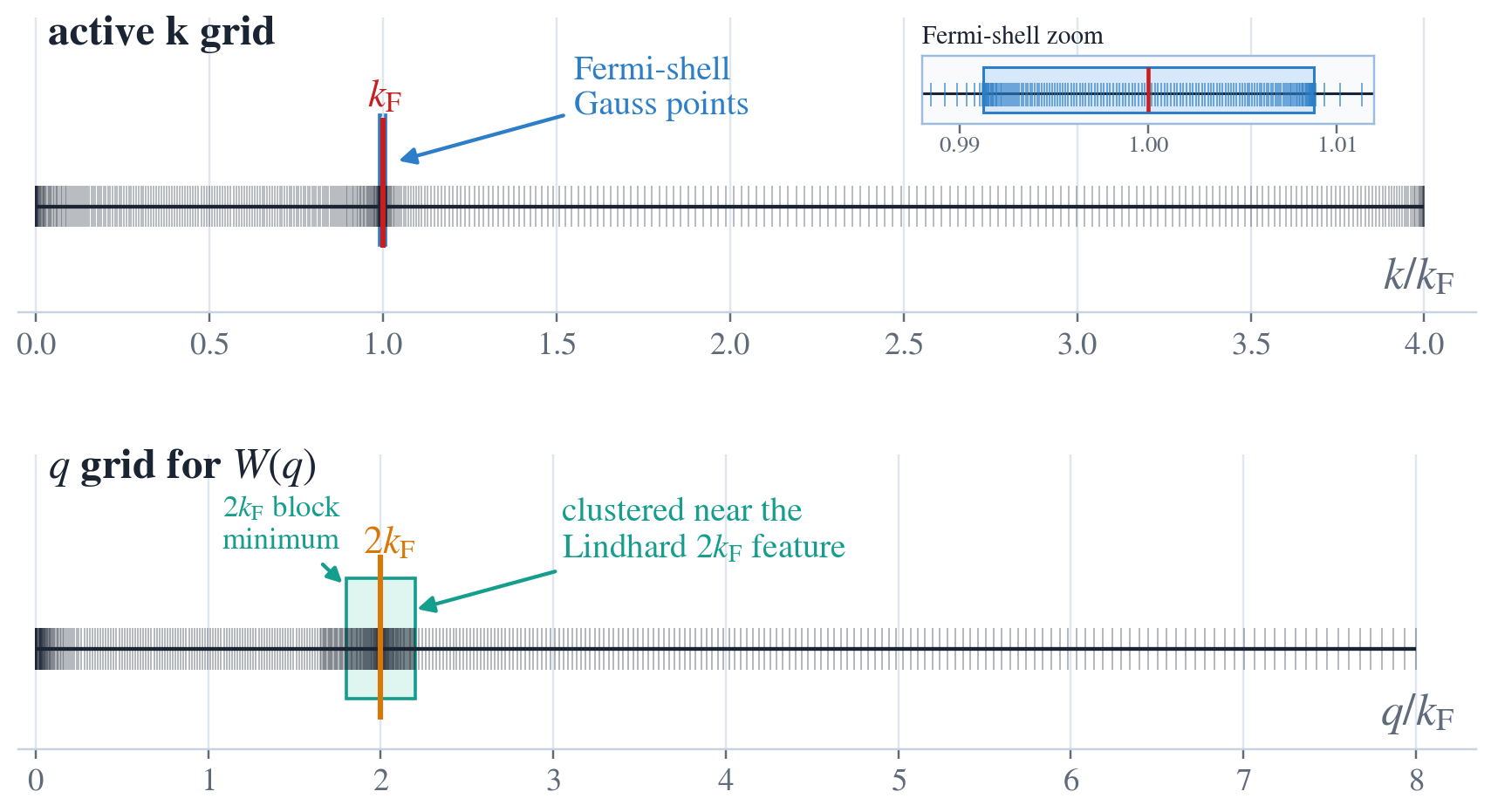
This representative grid is generated directly from migdal.grid for \(n=10^{20}\,\mathrm{cm}^{-3}\) and \(T=1\,\mathrm{K}\), with axes normalized by \(k_{\mathrm{F}}\). With the default point budgets this setup gives \(N_k=566\) and \(N_q=500\); each rug mark is an actual grid point. The active \(k\) grid concentrates points in the narrow thermal shell around \(k_{\mathrm{F}}\), which is why the figure includes a zoom inset. The \(q\) grid protects the region around \(2k_{\mathrm{F}}\), where the Lindhard polarization has its Kohn-feature structure, and then extends far enough to cover the radial convolution domain. The detailed Lindhard construction and RPA sign convention are explained in fixed-W0 polarization and the RPA sign convention.

If a smoke run fails its particle-number check, first increase the grid. Relax n0_check_atol only when you deliberately want a control-flow test rather than a physics result.

Interaction and diagonal cell averages

Keyword	Default / choices	Meaning
q_interp_mode	"q_singular" | "legacy"	Default "q_singular" splits the Coulomb-like \(A/q^2\) head before radial integration; this is the production path for long-range interactions and requires diagonal cell averages. "legacy" keeps the older piecewise-linear \(W(q)\) primitive, mainly for regression checks, old-result comparison, or isolating interpolation effects.
diag_average	"auto" | 1 | 0	Default "auto" turns diagonal cell averages on when q_interp_mode="q_singular" requires them; in legacy mode it follows the historical no-truncation rule. Use 1 to force averages and 0 only for controlled legacy or truncated diagnostics; q_singular rejects disabled averages.
diag_ncell	12	Quadrature cells for diagonal averages when a quadrature path is used.
diag_average_mode	"auto" | "analytic" | "gauss"	Default "auto" resolves to the analytic diagonal-cell formula for q_singular primitives and to Gauss quadrature otherwise. Use "analytic" explicitly for q_singular backend checks; use "gauss" for quadrature comparisons.
pi0_mode	"finite_T" | "0K" | "GG"	Default "finite_T" builds fixed \(W_0\) with the finite-temperature Lindhard polarization. "0K" uses the zero-temperature Lindhard formula, while "GG" builds the bubble numerically from \(G_0(\tau)G_0(\beta-\tau)\); this option is only for G0W0 and GW0 because ScGW updates \(\Pi\) self-consistently.
denom_policy	"sign_regularize" | "legacy_clip" | "fail" | "none"	Default "sign_regularize" only repairs denominators smaller than denom_min, preserving the local real sign or complex phase when possible. "fail" raises on such rows, "legacy_clip" replaces small denominators by a positive floor, and "none" leaves the denominator untouched.
denom_min	1.0e-10	Minimum denominator scale used by regularizing policies.
q_singular_head_policy	"pi_head" | "fit_w"	Default "pi_head" estimates the screened low-q head from the analytic polarization head. "fit_w" instead fits \(q^2 W\) from sampled low-q rows and is mainly a diagnostic for the singular-head construction.

In q_singular mode, diagonal cell averages are mathematically required for the exact diagonal radial block. The average changes only that self-cell quadrature block; it does not change the interaction definition. The table lists public driver choices; a lower-level "provided" head policy exists for callers that supply their own singular coefficient, but the public radial drivers reject it.

Normal-state SCF controls

GW0 solves G self-consistently with fixed W0. ScGW solves G, rebuilds the polarization bubble, and updates W.

Keyword	Common default / choices	Meaning
scf_conv_tol	1.0e-6	Max-norm tolerance for the gauge-invariant \(\Sigma-\mu\) residual.
scf_max_cycle	300	Maximum normal-state SCF cycles.
scf_damp	0.98	SCF damping/mixing control. 0.98 means mixing 2% new vector per cycle.
scf_diis_space	8	DIIS history size.
scf_diis_start_cycle	0	First cycle where DIIS may be used.
scf_continuation_max_dex	1.0	Maximum density-step size for restart-enabled continuation scans.
scf_mu_bracket	"nearest_positive" | "extreme"	Default "nearest_positive" chooses the closest positive-slope bracket around the current chemical-potential estimate. "extreme" uses the outer scan bracket and is a fallback for difficult density solves, but it is less local.
scf_fs_pin	True	Pin the Fermi-surface self-energy gauge when enabled.
scf_high_freq_density	True	Use the high-frequency corrected density formula in the SCF chemical-potential solve. Set to False only for direct \(-2G(\beta^-)\) endpoint comparisons.
allow_unconverged	False	Permit an unconverged SCF row to continue to the gap solve.

Disk checkpoints for the normal-state SCF loop are available through the Python driver API for GW0 and ScGW:

Keyword	Default	Meaning
scf_chkfile	None	HDF5 path for writing the latest SCF cycle state. Under MPI, only rank 0 writes.
scf_restart_chkfile	None	HDF5 path to load as the initial SCF guess for a later kernel() or scan() call.

The checkpoint stores the restart seed for the normal-state SCF loop: sigma, mu, the optional Fermi-surface pin shift, the active k grid, the Matsubara grid, and basic diagnostics. It does not serialize DIIS history, the gap solve, or the derived scGW W/polarization tables. Use it to resume the same GW0/scGW method on the same temperature and grid after an interruption. In a density scan with scan(restart=True), the file can seed the first point; once the scan has an in-memory continuation seed, that seed takes precedence.

ScGW also has polarization and tail controls. Keep these defaults for tutorial runs unless you are doing a specific stability audit.

Keyword	Default / choices	Meaning
n_tail	100	Minimum number of passive k points in the separate polarization integration tail.
sigma_tail_policy	"exchange_static" | "exchange_t0" | "zero"	Default "exchange_static" fills the passive tail with a finite-temperature static-exchange estimate. "exchange_t0" uses the \(T=0\) exchange expression, while "zero" leaves the passive tail empty apart from the gauge shift.
pi_imag_policy	"warn" | "fail"	Default "warn" logs imaginary-part diagnostics in the polarization bubble and continues. "fail" turns the same diagnostic into an exception for stricter audits.
pi_positive_policy	"warn" | "fail"	Default "warn" reports positive real entries of \(\Pi\) above tolerance and continues. "fail" stops the row when that sign diagnostic is violated.
pi_positive_action	"keep" | "zero_small"	Default "keep" leaves small positive \(\Pi\) entries unchanged after diagnostics. "zero_small" zeros only positive entries below pi_positive_tol.
pi_low_q_policy	"asymptotic" | "none"	Default "asymptotic" continues the low-q polarization using the expected small-q behavior before building \(W\). "none" uses the sampled values directly.
q_low_factor, q_static_low_factor	2.0e-2, None	Low-q continuation thresholds in units of \(k_{\mathrm{F}}\). q_static_low_factor=None reuses q_low_factor.
allow_no_pi_tail	False	Permit a run without a passive polarization tail. This is mainly for controlled tests, not production-style scGW scans.

With the default pi_low_q_policy="asymptotic", finite bosonic frequencies are continued as \(\Pi(q,\mathrm{i}\nu_n)\propto q^2\) below \(q_{\mathrm{low}} k_{\mathrm{F}}\), where \(q_{\mathrm{low}}\) is q_low_factor; the static component is held at its reference low-q value below \(q_{\mathrm{static,low}} k_{\mathrm{F}}\), with \(q_{\mathrm{static,low}}\) set by q_static_low_factor. The detailed formulas are in scGW low-q continuation.

The table above lists driver constructor defaults. Some scripts in the recommended example order choose more conservative defaults for long scans, especially continuation step sizes and scGW cycle limits. Use python examples/<name>/run.py --help when you need the script-level defaults.

Advanced debug-only gap options check_precond and check_precond_nsamples are available through the Python driver kwargs but are not part of the common package CLI. The package CLI exposes scf_high_freq_density only indirectly for scGW: --legacy-scf-density switches scGW to the direct endpoint density convention. The package CLI --restart option controls in-memory scan continuation; disk SCF checkpoint paths are currently Python driver keywords.

Gap solver

The radial gap problem is solved by PySCF’s Davidson solver. Driver keyword arguments are passed through to GapConfig.

Keyword	Default / choices	Meaning
truncate	False	Restrict the active Matsubara window.
wcut	driver-derived	Frequency cutoff when truncation is enabled.
precond	"even_diag" | "ones"	Default "even_diag" uses the even-frequency diagonal estimate as the Davidson preconditioner. "ones" is an identity preconditioner, useful mostly for debugging whether the preconditioner is affecting convergence.
cache	"auto" | "off"	Default "auto" materializes radial matvec geometry when the memory policy allows it. "off" streams the geometry instead, which can be slower but is useful for memory audits.
davidson_tol	1.0e-6	Davidson convergence tolerance.
davidson_max_cycle	300	Maximum Davidson cycles.
davidson_max_space	20	Davidson subspace limit.
nroots	1	Number of Davidson roots requested from the gap solver. Keep 1 unless you are explicitly comparing leading and subleading gap channels.
return_gap_function	False	Return the full scaled gap function for diagnostics.

The reported pairing strength is

\[ \lambda = -\operatorname{Re}(\eta_{\mathrm{selected}}), \]

where \(\eta_{\mathrm{selected}}\) is the selected raw Davidson eigenvalue.

Takada projection controls

TakadaProjection is separate from the sparse-IR radial drivers. Its main controls are the dense angular grid, the dimensionless energy grid, and the kernel symmetry check.

Keyword	Default	Meaning
n_q, n_theta	20, 12	Quadrature sizes for the projected dense kernel.
x_core, x_max	1.0e-5, 1.0e3	Inner and outer limits for the dimensionless energy grid.
n_neg, n_pos	48, 52	Occupied and unoccupied energy-grid counts.
max_symmetry_error	1.0e-10	Maximum allowed projected-kernel symmetry error.